Fitting Generative Network Models

The likelihood that a Generative Network Model will produce a particular network is controlled by parameters \(\eta\) and \(\gamma\) which determine how the distance and affinity transforms, \(d\) and \(k\), are derived from the distance and affinity matrices, \(D\) and \(K\). As discussed above, it is very hard to compute in general the likelihood that any given parameter pair (and generative rule) will output a particular weight matrix. Instead, the parameters of the GNM are typically fit by generating many networks for each choice of parameters, and asking which choice of parameters produces networks that whose topology most accurately matches that seen in real brain networks. This section outlines the fitting procedure by which we determine which parameters give the best match to empirical data.

Kolmogorov-Smirnov Measures of Topological Fit

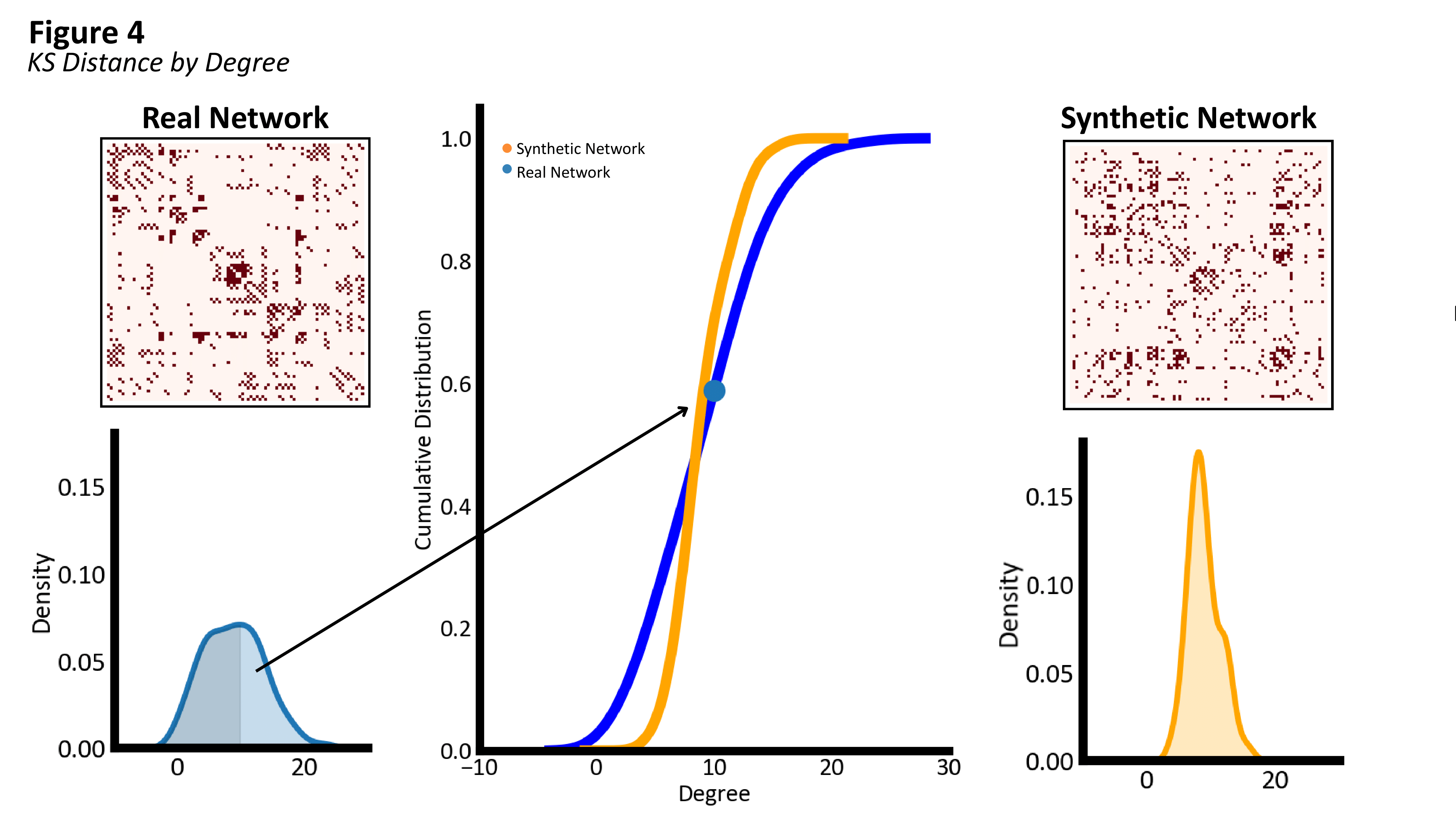
A distribution describes the collection of values taken by a particular network measure across all elements in a network. For instance, the degree distribution is the degree of each node in the network, whilst the edge length distribution is the distance spanned by each edge in the network. One way of measuring similarity between networks is to measure the similarity between the distributions of various network measures between the networks.

To compare distributions between synthetic and empirical networks, we use the Kolmogorov-Smirnov (KS) distance between those distributions. The KS distance begins with the cumulative distribution functions for each of the two distributions. A cumulative distribution function at a given point is the fraction of values in the distribution that are less than or equal to that point. For example, if we have degrees of 1, 3, 5, 7, and 9 across five nodes, the CDF at the point 5 would be 0.6, since three out of five values (1, 3, and 5) are less than or equal to 5. From the CDF for the synthetic and empirical distribution over network properties, the KS distance can then be computed as the maximum difference between the CDFs. $$ \mathrm{KS} = \max_x | F_{\mathrm{empirical}}(x) - F_{\mathrm{synthetic}}(x) | $$ The KS distance ranges from 0 (identical distributions) to 1 (completely different distributions).

For any two networks we wish to compare (i.e., empirical and synthetic), we can obtain a KS distance for each network measure of interest. For example, we may compute the degree KS distance and the clustering coefficient KS distance. Note that these distances are in general different; networks can have a very similar distribution of degrees while having very different distributions of clustering coefficients. Below, we give various network measures for which we typically compute the KS distance when attempting to fit the parameters of a binary GNM.

Statistics for Binary Network Fitting

There are four network statistics typically used to quantify fit between an empirical and synthetic network in the GNM: degree, clustering coefficient, betweenness centrality, and edge length.

The degree of a node is equal to the total number of connections that node has, \(s_i = \sum_j A_{ij}\). The degree distribution across all nodes in a network can reveal whether there is roughly uniform level of connectivity between all nodes in the network, of if some nodes have much higher connectivity than others. See Node-Level Measures for a more detailed explanation of degree.

The clustering coefficient, \(c_i\) of a node measures the extent to which its neighbours are also connected to each other, quantifying local network clustering. It is equal to the fraction of possible connections between a node's neighbours that are actually present. See Node-Level Measures for a more detailed explanation of clustering coefficients.

Betweenness centrality quantifies how often a node sits on the shortest paths between other nodes in the network. The betweenness centrality of a node \(i\) is the fraction of pairs of other nodes in the network for which the shortest paths between those nodes passes through \(i\). See Node-Level Measures for a more detailed explanation of betweenness centrality.

Finally, the edge length of an edge represents the physical distance between nodes connected by that edge. In particular, if \(i\) and \(j\) are connected (i.e., \(A_{ij} = 1\)), then the edge length of their connection is \(D_{ij}\) where \(D\) is the distance matrix. The edge length distribution typically shows an overrepresentation of short connections compared to what would be expected from random wiring, reflecting the influence of spatial constraints on network formation.

Statistics for Weighted Network Fitting

The above network measures can be adapted to the case where we wish to instead measure the difference between weighted networks. When working with weighted networks, connection strengths are typically normalised before computing network statistics to ensure meaningful comparisons between networks with different overall weight scales. Normalisation is performed by dividing each individual weight by the maximum weight within the network: \(W'_{ij} = \frac{ W_{ij} }{ \max_{ab} W_{ab} }\). This ensures that all weights fall within the range [0,1] whilst preserving the relative relationships between connection strengths. Without this normalisation, networks with systematically higher weights would appear different even if their relative weight patterns were identical.

Weighted node strength extends the concept of degree to weighted networks by summing the weights of all connections attached to a node rather than simply counting them. It is computed analogously as \(s_i = \sum_j W_{ij}\). This measure captures not only how many connections a node has, but also how strong those connections are.

Weighted betweenness centrality adapts the concept of betweenness centrality to weighted networks by considering the weights of edges when computing shortest paths. Rather than counting the number of edges in a path, weighted betweenness centrality modifies the lengths of paths according to the weighting used along those paths.

Weighted clustering coefficient generalises local clustering to weighted networks by incorporating the weights of connections within local neighbourhoods. This measure captures not only whether a node's neighbours are connected to each other, but also how strongly they are connected.

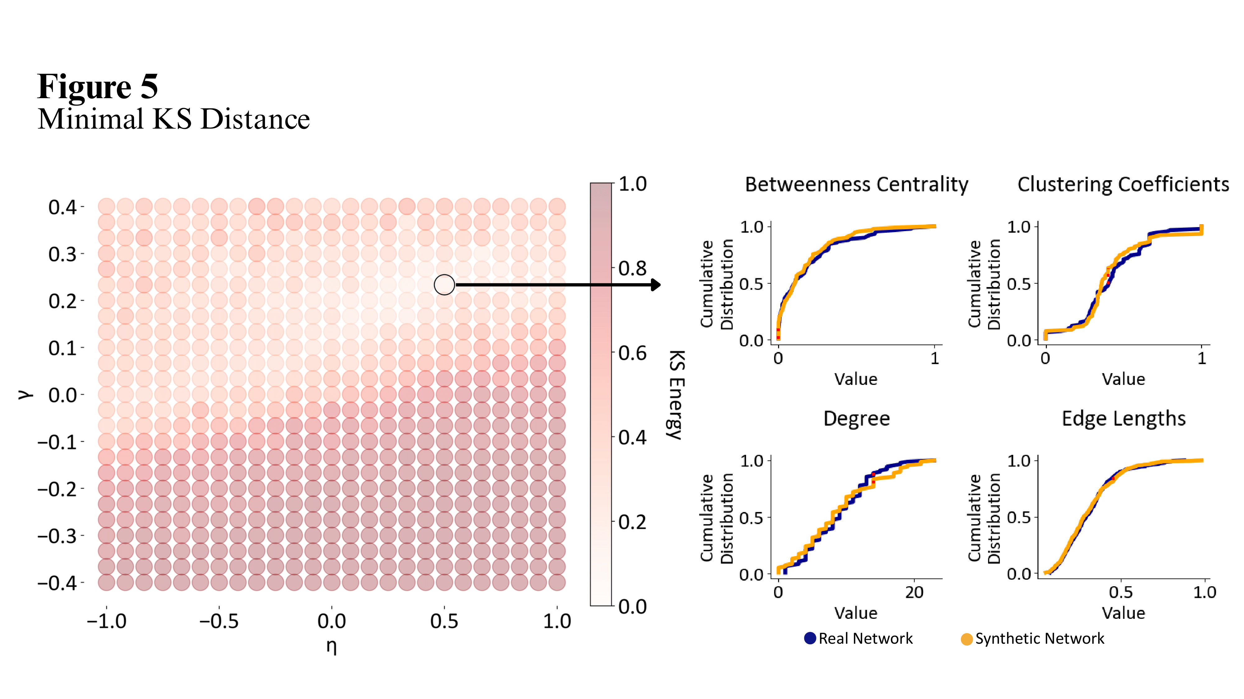
Energy

Having computed a set of KS distances for a variety of network measures, we combine them into a single measure called the energy. The for binary networks, the energy is defined as $$ E = \max\left( \text{KS}_{\text{degree}}, \text{KS}_{\text{clustering}}, \text{KS}_{\text{betweenness}}, \text{KS}_{\text{edge length}} \right), $$ where each KS term represents the Kolmogorov-Smirnov distance between the distributions of that property in the synthetic and empirical networks. Lower energies indicate better agreement between the network topology generated by the model and the real network topology.

For weighted networks, energy is computed similarly but uses weighted versions of network properties and excludes edge length (since this is a property of the spatial embedding rather than the weight structure): $$ E_{\text{weighted}} = \max\left( \text{KS}_{\text{strength}}, \text{KS}_{\text{weighted clustering}}, \text{KS}_{\text{weighted betweenness}} \right). $$ The maximum operation ensures that achieving low energy requires the synthetic networks to match the real networks in all properties; a low energy cannot be achieved by excelling in one property whilst performing poorly in others.

Implementation details for energy computation can be found in the gnm.evaluation module, which provides comprehensive evaluation criteria for both binary and weighted networks.

Correlational Measures of Topographical Fit

Except for edge length, the network statistics computed for the KS distances which comprise the energy are all purely topological, in the sense that they are agnostic to the identities of the nodes in the network. Because KS distance measures only the difference between distributions, two networks may have a very low degree KS distance while the nodes with a high degree in the first network may be the nodes with a low degree in the second network. Ideally, we would like our GNM to not only capture the topological properties of real brain networks, but also their topographical properties - in other words, the models should place particular features in the right place.

To capture topographical fit, we use the correlation between node-level properties between the two networks. In other words, if the property is large for a node in one network, it ought to be large for the other node as well. While the goal is to match nodes exactly, matching to nearby nodes is also good. As such, we typically apply spatial smoothing to the network properties in which the propery is averaged over nearby nodes. Specifically, for a node-level network property \(X_i\), the unnormalised spacial smoothing weights \(\tilde{\Omega}\) are given by $$ \tilde{\Omega}_{ij} = \exp\left(-\frac{D_{ij}^2}{2\sigma^2}\right). $$ For each node \(i\), a larger weight is assigned to those nodes \(j\) which are closer to \(i\) in space (i.e., have a lower value of \(D_{ij}\)). The parameter \(\sigma\) controls the spatial scale of the smoothing. These weights do not sum to \(1\), so we normalise by performing $$ \Omega_{ij} = \frac{\tilde{\Omega}_{ij}}{\sum_k \tilde{\Omega}_{ik} }. $$ The node-level property is then smoothed using these weights to obtain $ \sum_j \Omega_{ij} X_j $. The correlation between these smoothed quanties across the two networks quantifies the degree of topographical fit.

The properties used for correlational fit measures are the same as those used for binary KS fit: degree, clustering, and betweenness centrality.

Parameter Sweeps

Now that we have specified a method for specifying the level of agreement between empirical and model-generated networks, we can describe how to find the parameter set which reliably produces networks that have the best fit. This is done by searching over the parameter space to find configurations that have the best average fit between the empirical network and the model-generated networks. This search encompasses not only continuous parameters like \(\eta\) and \(\gamma\), but also discrete choices such as which generative rule to use for computing the affinity matrix or which loss function to optimise for weighted GNMs.

The stochastic nature of GNMs introduces additional complexity into parameter fitting. The same parameter configuration will in general produce different networks across multiple simulation runs due to the probabilistic sampling of connections. To account for this variability, it is necessary to generate many networks from each parameter set and aggregate the fit measures across these simulations. Common aggregation methods include computing the mean energy across simulations, which provides a stable estimate of expected performance, and quantile aggregation, which can focus on typical or best-case performance. The median represents a special case of quantile aggregation at the 50th percentile, offering robustness to outlier simulations with unusually poor fit or unusually good fit.

Grid searches involve systematically sweeping over the parameter space by evaluating the model at regularly spaced parameter combinations. The coarseness or fineness of the grid determines the resolution of the search, with finer grids providing more thorough exploration at the cost of increased computational requirements. Grid searches are particularly suitable when the parameter space is low-dimensional and computational resources allow for exhaustive evaluation.

Algorithm: Grid Search for Parameter Fitting

Input: Parameter ranges, grid resolution, number of simulations per parameter set

For each parameter combination in the grid do:

1. For each run in the batch do:
   • Generate new synthetic network using current parameters.
   • Compute energy between synthetic and empirical network.
2. Aggregate energy across all simulations in the batch (using, *e.g.*, the mean or median energy for the batch).
3. Store aggregated energy for current parameter combination,

End for

Return: Parameter combination with lowest aggregated energy.

Bayesian optimisation methods provide a more sophisticated method to search parameter space in which an estimate of the dependence of the energy on parameter values is formed based on previously observed energy values. This model can then guide the search toward promising regions of parameter space, increasing the efficiency of the search process over the exhausive enumeration used by grid search. These methods are particularly valuable when the search space becomes very large, as they can achieve good results with fewer parameter evaluations than grid searches. The downside is that they are non-exhausive, and as such there is always a possibility that the optimal parameter combination was not found by the model. For comprehensive guidance on Bayesian optimisation techniques and implementations, see relevant Weights & Biases documentation.

Implementation details for parameter sweeps can be found in the gnm.fitting module, which provides tools for both grid search and Bayesian optimisation approaches to model fitting.